rm(list=ls())
df <- read.csv('https://www.dropbox.com/scl/fi/rzu7r7c64dr1o3rr2j444/wk9_1.csv?rlkey=zt3a7hp97no5on5zhdezbkszl&dl=1')81 Linear Models for Regression - Practical
81.1 Theory
The linear regression model expresses a linear relationship between the dependent variable (target) \(y\) and one or more independent variables (features) \(X\).
In its simplest form (simple linear regression), the model is expressed as \[ y=β 0 +β 1 x+ϵ \] where:
\(y\) is the dependent variable.
\(x\) is the independent variable.
\(β0\) is the intercept.
\(β1\) is the slope coefficient.
\(ϵ\) is the error term.
The objective in linear regression is to find the line of best fit that minimises the difference between the predicted and actual values.
Coefficients (\(β\)) are estimated using training data. The goal is to find the values of \(β0\) and \(β1\) that minimise the residual sum of squares (RSS), which is the sum of squared differences between observed and predicted values.
Linear regression assumes linearity (relationship between the dependent and independent variables should be linear), independence (observations should be independent of each other), homoscedasticity (residuals (errors) should have constant variance across all levels of the independent variables) and normality (residuals should be normally distributed).
The ‘goodness of fit’ of a linear regression model is typically assessed using the coefficient of determination (R2), which measures the proportion of variance in the dependent variable that is predictable from the independent variable(s).
Once the model is fitted and the coefficients are estimated, it can be used to make predictions. The predicted value of \(y\) for a given \(x\) is calculated by plugging the values of \(x\) into the model equation.
Multiple linear regression extends simple linear regression to multiple independent variables.
81.2 Demonstration
Process
![]()
Load dataset
Feature selection
From the dataset, I can identify eight IVs (predictor variables):
players_age: Age of the player (integer).
team_experience: Years of experience in the current team (integer).
average_points: Average points per game (integer).
average_assists: Average assists per game (integer).
average_rebounds: Average rebounds per game (integer).
player_position: Player position, encoded from 1 (point guard) to 5 (center) (integer).
injury_history: Whether the player has a significant injury history (0: no, 1: yes) (dichotomous).
free_throw_accuracy: Free throw accuracy percentage (continuous).
I can also identify three possible DVs (outcomes, or dependent variables):
mvp_votes: Number of MVP votes received (integer).
all_star: Whether the player was an All-Star (0: no, 1: yes) (dichotomous).
championship_win: Whether the player’s team won the championship (0: no, 1: yes) (dichotomous).
In this case, I am interested in predicting how many ‘Most Valuable Player’ votes a player receives; my outcome is continuous. Linear regression is therefore an appropriate model for this kind of question.
Normalise data
Normalising a dataset is usually essential in ML, as it scales the ranges of the features, making it easier for ML algorithms to converge. Normalisation scales the data on a range of 0 to 1.
I could also standardise the data, giving it a mean of 0 and sd of 1.
In this example, I’m going to normalise all of the data, as my outcome variable is continuous rather than dichotomous. I could also standardise the data, and examine the difference this makes to the model.
# i paste in my normalise function
normalise<- function(x) {
  return ((x - min(x)) / (max(x) - min(x)))
}

df_norm <- as.data.frame(lapply(df, normalise)) # create new dataframe
Split the data into training and testing sets
In ML, we usually want to split our dataset into two parts; training and testing.
We train our model on the first dataset, and test it on the second. This prevents the issue of overfitting (our model is ‘too good’).
# first, calculate what number represents 80% of the dataset
sample_size <- floor(0.8 * nrow(df_norm))
# then create that number of indices
train_indices <- sample(seq_len(nrow(df_norm)), size = sample_size)

# create new dataframe by extracting the observations at those rows
train_data <- df_norm[train_indices, ]

# create another dataframe by extracting the observations that are NOT at those rows.
test_data <- df_norm[-train_indices, ]
Here, I’ve split the dataset into training (80%) and testing (20%) sets to evaluate our model’s performance.
Specify the model
My task is to use linear regression to explore whether it’s possible to accurately predict the mvp_votes, based on the predictor variables. I’m asking which factors are most predictive of the number of votes received, and what is their relative role?
For this model, I’m going to ‘go big’ and plug all my predictors in at once. My model will be:
mvp_votes ~ players_age + team_experience + average_points + average_assists + average_rebounds + player_position + injury_history + free_throw_accuracy
Run the linear regression model
Now I run that regression model on the training dataset. Note that I’ve asked for the AIC to be output at the end, which will give me a way of comparing different models.
# fit model
model <- lm(mvp_votes ~ players_age + team_experience + average_points + average_assists + average_rebounds + player_position + injury_history + free_throw_accuracy, data = train_data[, -ncol(train_data)])

# summarise model
summary(model)
Call:
lm(formula = mvp_votes ~ players_age + team_experience + average_points +
    average_assists + average_rebounds + player_position + injury_history +
    free_throw_accuracy, data = train_data[, -ncol(train_data)])

Residuals:
     Min       1Q   Median       3Q      Max
-0.38087 -0.08183 -0.00477  0.07708  0.51440

Coefficients:
                      Estimate Std. Error t value Pr(>|t|)
(Intercept)          1.143e-01  2.624e-02   4.354 1.61e-05 ***
players_age         -1.369e-02  1.928e-02  -0.710    0.478
team_experience     -1.851e-02  1.985e-02  -0.932    0.352
average_points       3.486e-01  2.003e-02  17.404  < 2e-16 ***
average_assists      2.078e-01  2.003e-02  10.374  < 2e-16 ***
average_rebounds    -1.316e-02  1.981e-02  -0.665    0.507
player_position      8.522e-03  1.862e-02   0.458    0.647
injury_history      -3.200e-01  1.281e-02 -24.974  < 2e-16 ***
free_throw_accuracy -7.447e-05  1.985e-02  -0.004    0.997
---
Signif. codes:  0 '***' 0.001 '**' 0.01 '*' 0.05 '.' 0.1 ' ' 1

Residual standard error: 0.1299 on 514 degrees of freedom
Multiple R-squared:  0.679, Adjusted R-squared:  0.674
F-statistic: 135.9 on 8 and 514 DF,  p-value: < 2.2e-16
# calculate and print AIC
aic_value <- AIC(model)
print(aic_value)[1] -639.9181I’ve used the
lmfunction to build a linear regression model, using the training set.
Check model fit
If we have some predictive variables that do not seem to be significant, we can explore what happens to model accuracy when we remove them from the linear regression.
Note that the AIC is lower for this model (for the AIC, lower = better).
model2 <- lm(mvp_votes ~ average_points + average_assists + injury_history, data = train_data)
summary(model2)
Call:
lm(formula = mvp_votes ~ average_points + average_assists + injury_history,
    data = train_data)

Residuals:
     Min       1Q   Median       3Q      Max
-0.38820 -0.08026 -0.00575  0.07542  0.52238

Coefficients:
                Estimate Std. Error t value Pr(>|t|)
(Intercept)      0.09616    0.01549   6.209 1.09e-09 ***
average_points   0.34835    0.01993  17.479  < 2e-16 ***
average_assists  0.20597    0.01971  10.449  < 2e-16 ***
injury_history  -0.31960    0.01268 -25.214  < 2e-16 ***
---
Signif. codes:  0 '***' 0.001 '**' 0.01 '*' 0.05 '.' 0.1 ' ' 1

Residual standard error: 0.1295 on 519 degrees of freedom
Multiple R-squared:  0.6778,    Adjusted R-squared:  0.6759
F-statistic: 363.9 on 3 and 519 DF,  p-value: < 2.2e-16
aic_value <- AIC(model2)
print(aic_value)[1] -647.8565Apply to testing data
Now, I’m going to use the second model I built (model2) to predict the number of MVP votes I can expect to find using my predictive model.
predictions <- predict(model2, test_data)Examine predictions
There are a few different visualisations that can help us explore how the model’s predictions compared to the actual outcomes in the test data:
library(ggplot2)
plot(test_data$mvp_votes, predictions, xlab = "Actual MVP Votes", ylab = "Predicted MVP Votes", main = "Actual vs. Predicted MVP Votes")
abline(0, 1, col = "red")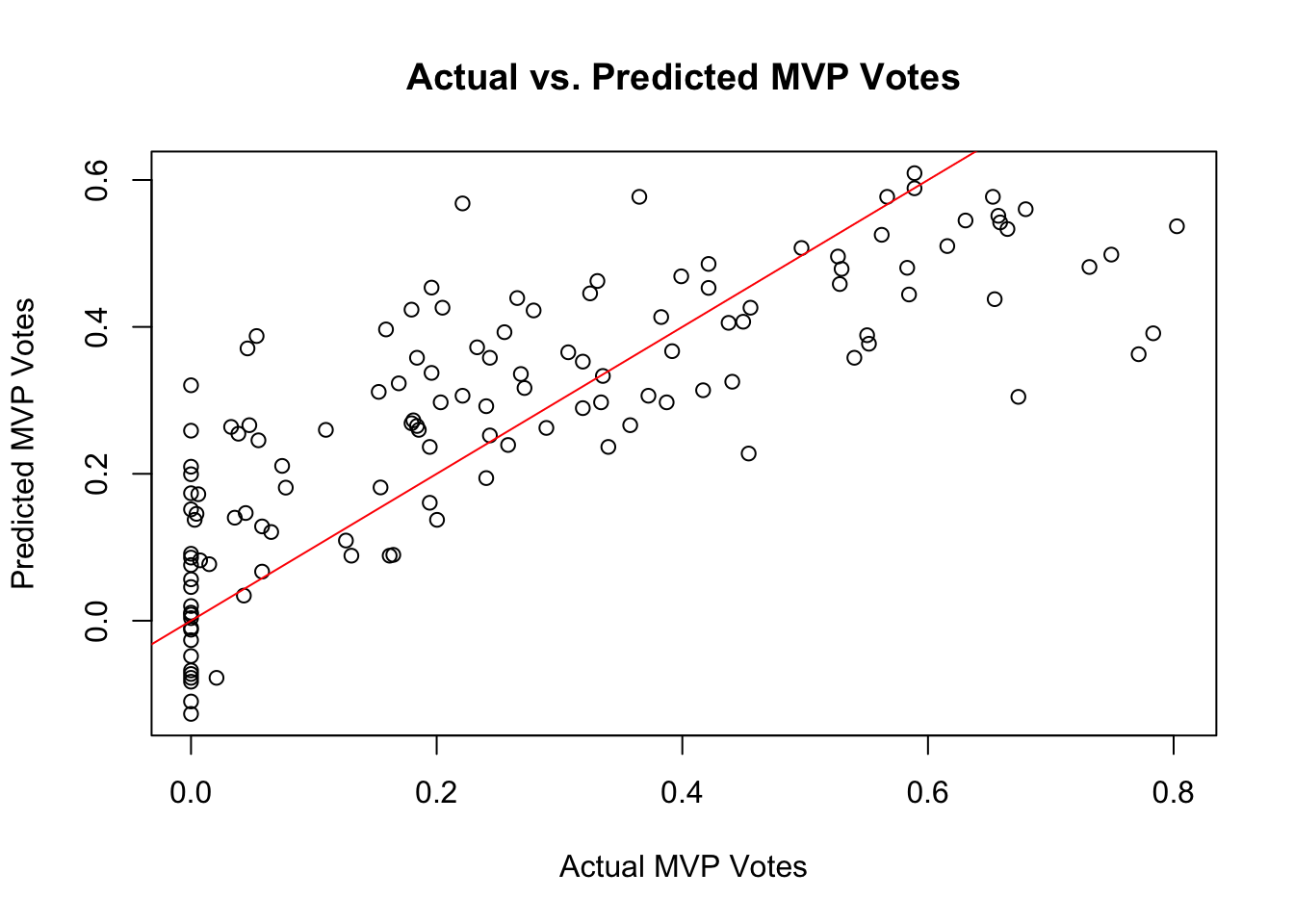
residuals <- test_data$mvp_votes - predictions
# Residual Plot
plot(test_data$mvp_votes, residuals, main = "Residuals vs. Actual Values",
xlab = "Actual Values", ylab = "Residuals", pch = 4)
abline(h = 0, col = "red") # add horizontal line at 0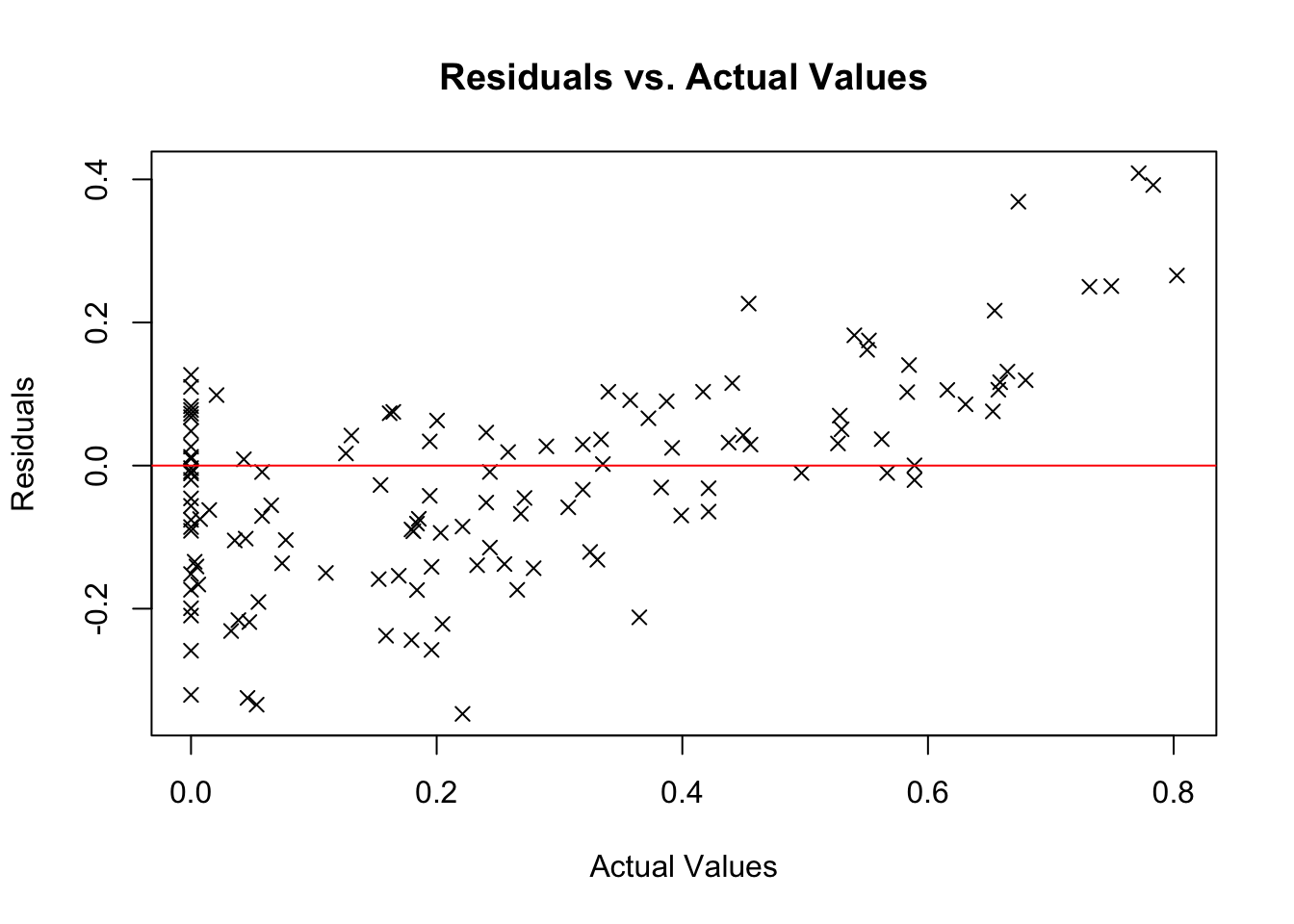
test_data$predicted <- predictions
# Scatter plot
ggplot(test_data, aes(x = mvp_votes, y = predicted)) +
geom_point() +
geom_abline(intercept = 0, slope = 1, color = "red", linetype = "dashed") +
labs(title = "Actual vs. Predicted Values",
x = "Actual Values",
y = "Predicted Values") +
theme_minimal()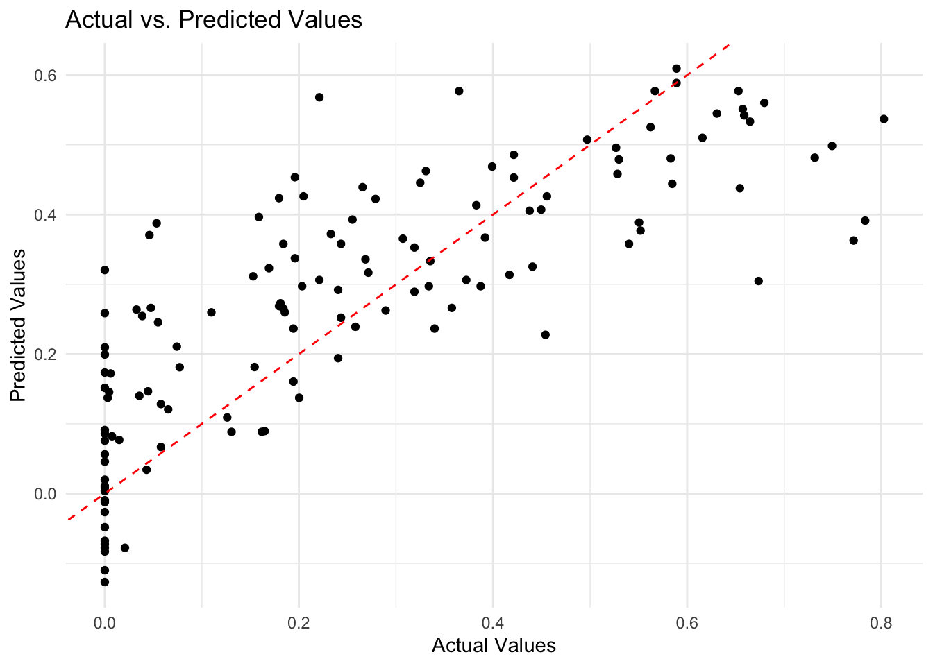
I’ve created a scatter plot to compare actual vs. predicted
mvp_votesvalues. The red line represents a perfect prediction.
81.3 Practice
Repeat the steps above on the following F1 dataset.
Your task is to create a model to predict the RacePosition based on the predictor variables. Which predictor variables are significant, and to what extent does your model explain the variance in the observed data?
rm(list=ls())
df <- read.csv('https://www.dropbox.com/scl/fi/4huhvcj21dlizwso430ma/wk9_2.csv?rlkey=2f5j7kg68rgkimuduz6j3tm8v&dl=1')show solutions
### Normalise
normalise<- function(x) {
return ((x - min(x)) / (max(x) - min(x)))
}
df_norm <- as.data.frame(lapply(df, normalise))
### Run regression model
#### Split into training and testing sets
sample_size <- floor(0.8 * nrow(df_norm))
train_indices <- sample(seq_len(nrow(df_norm)), size = sample_size)
train_data <- df_norm[train_indices, ]
test_data <- df_norm[-train_indices, ]
#### Fit linear model
model <- lm(RacePosition ~ CarPerformanceIndex + QualifyingTime + DriverAge + EnginePower + TeamExperience + WeatherCondition + CircuitType + PitStopStrategy, data = train_data[, -ncol(train_data)])
summary(model)
aic_value <- AIC(model)
print(aic_value)
#### Different models
model2 <- lm(RacePosition ~ CarPerformanceIndex + QualifyingTime + EnginePower + PitStopStrategy, data = train_data)
summary(model2)
aic_value <- AIC(model2)
print(aic_value)
predictions <- predict(model2, test_data)
### Visualise actual vs. predicted data
plot(test_data$RacePosition, predictions, xlab = "Actual Race Position", ylab = "Predicted Race Position", main = "Actual vs. Predicted Race Position")
abline(0, 1, col = "red")
#### More plots
# Residuals vs. Fitted Values
plot(model2, which = 1)